The case we are handling: a 2 layers network

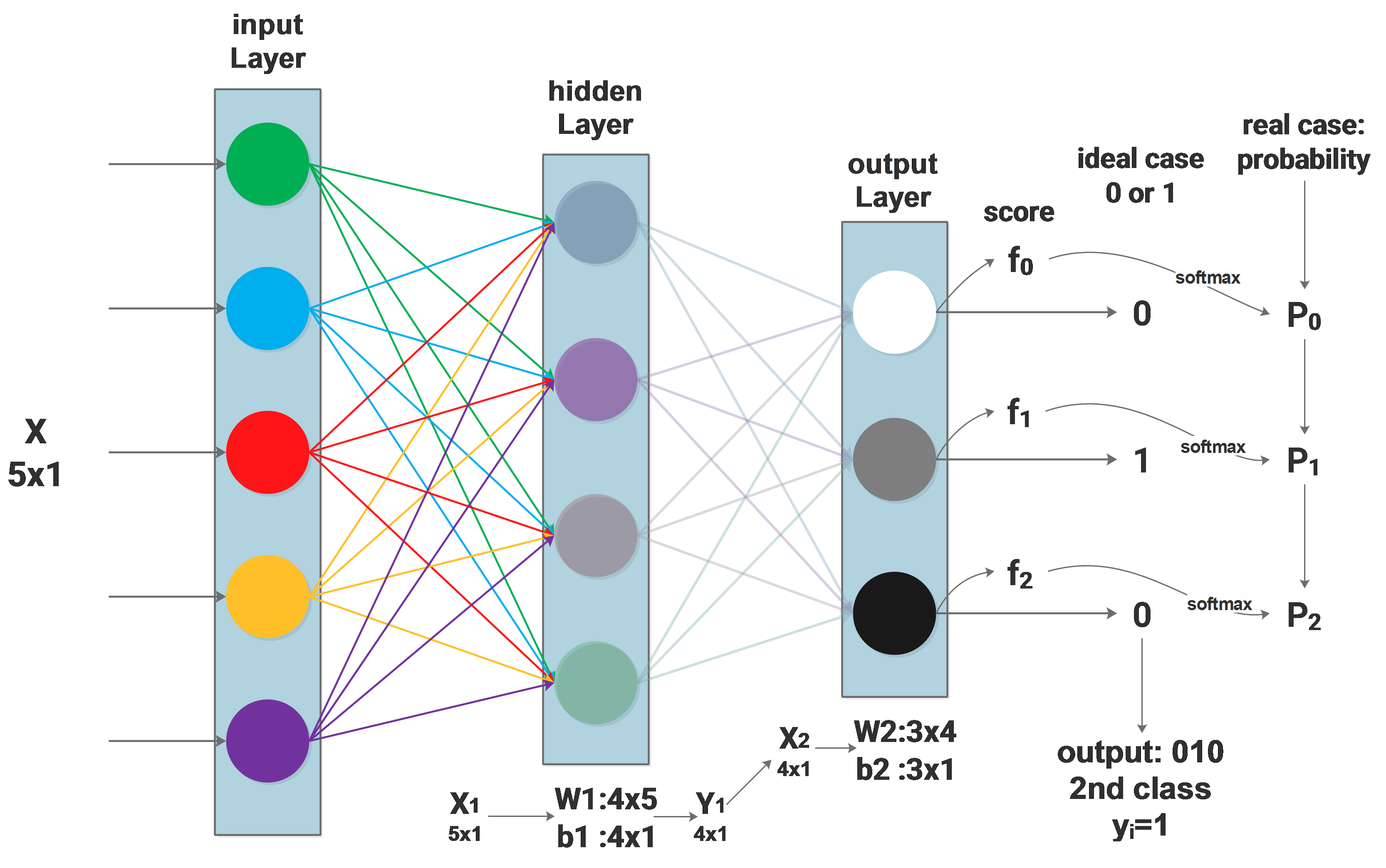
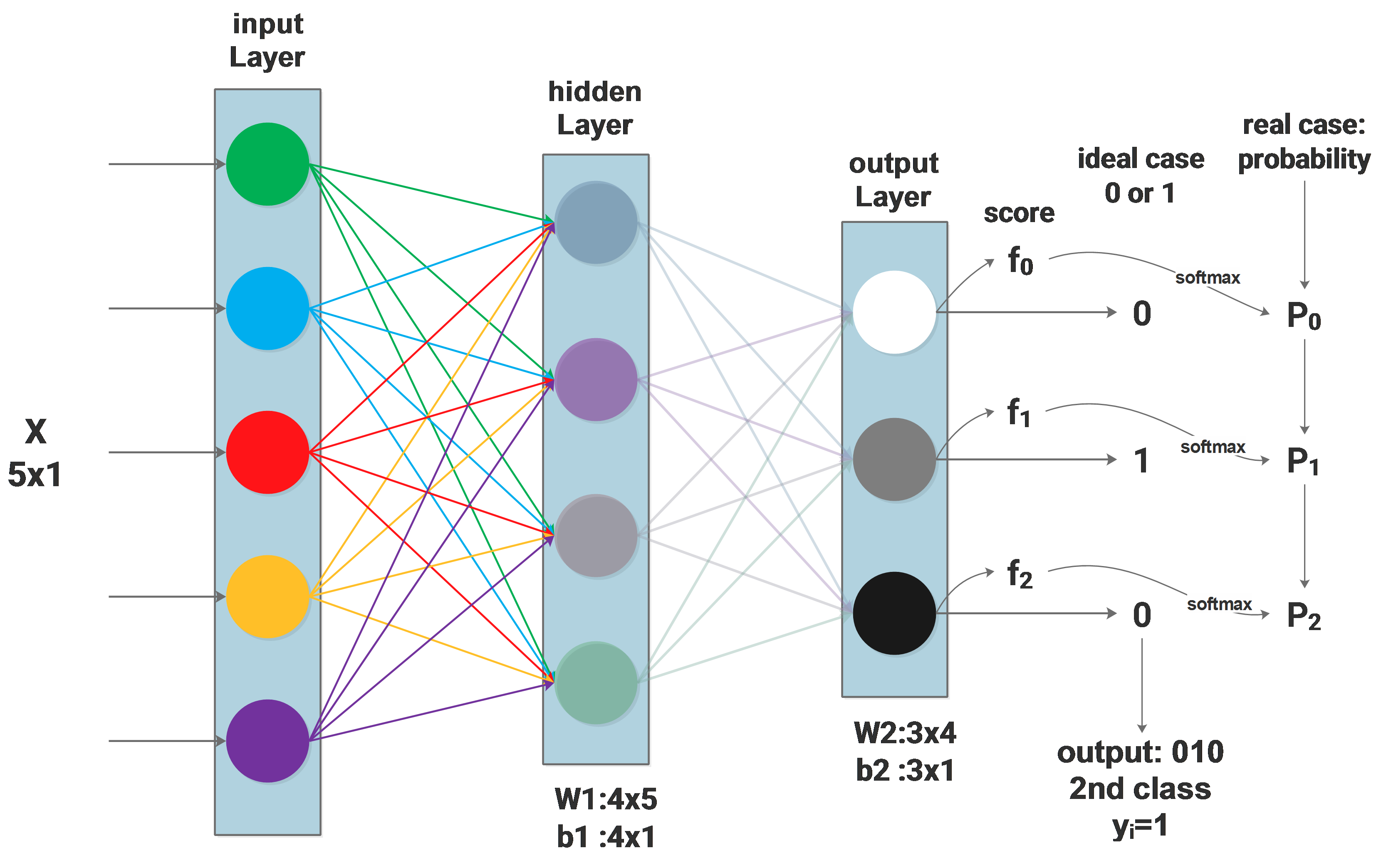
Background:the network and symbols

Firstly the network architecture will be described as:

Dropout regularization

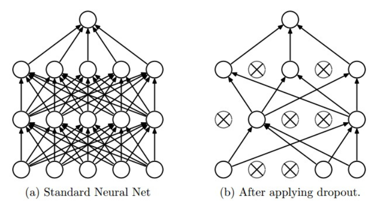
Dropout is a commonly used regularization method, it can be described by the diagram below: only part of the neurons in the whole network are updated. Mathematically, we apply some possibility \(p\)(we use 0.5) to a neuron to keep it active or keep it asleep:

Weight Initialization

All-Zero Initialization

It is easy to think that we set all the weights to be zero, but it’s terribly wrong, cause using all zero initialization will make the neurons all the same during the backpropagation update. We don’t need so many identical neurons. Actually, this problem always exists if the weights are initialized to be the same.

Small random values

One guess to solve the problem of all-zero initialization is setting the weights to be small random values, such as \(W=0.01*np.random.randn(D,H) ​\) . It is also problematic because very small weights cause very small updates and the update values become smaller and smaller during the backpropagation. In the deep network, this problem is very serious as you may find that the upper layers never update.

The LSVM (SVM with latent variable) is mostly used for human figure detection, it is very efficiency because it puts the human figure’s structure into consideration: a human figure has hands, head and legs. The LSVM models the human figure structure with 6 parts, and the position of these 6 parts are latent value.

The basic logic is sliding a window on the image, for every position we get a small image patch, by scoring this image patch we can predict whether this image patch contains a human figure or not.

Defining the score function

Anyway, the first thing to do: defining a score function:

Structural SVM is a variation of SVM, hereafter to be refered as SSVM

Special prediction function of SSVM

Firstly let’s recall the normal SVM’s prediction function:

\[f(x)=sgn((ω\cdot x)+b)\]

ω is the weight vector，x is the input，b is the bias，\(sgn\) is sign function，\(f(x)\) is the prediction result.

On of SSVM’s specialties is its prediction function：

\[f_ω (x)=argmax_{y∈Υ} [ω\cdot Φ(x,y)]\]

y is the possible prediction result，Υ is y’s searching space，and Φ is some function of x and y.Φ will be a joint feature vector describes the relationship between x and y

Then for some given \(\omega\), different prediction will be made according to different x.

Sepp Hochreiter was graduated from Technische Universität München, LSTM was invented when he was in TU and now he is the head of Institute of Bioinformatics, Johannes Kepler University Linz.

Today he comes by Munich and gives a lecture in Fakultät Informatik.

At first, Hochreiter praised how hot is Deep Learning (to be referred as DL) around the world these days, especially LSTM, which is now used in the new version of google translate published a few days ago. The improvements DL made in the fields of vision and NLP are very impressive.

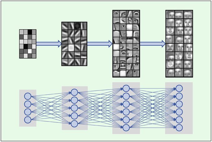
Then he starts to tell the magic of DL, taking face recognition as an example, the so-called CNN (Convolution Neuro Networks):

Centering and Scaling