Uncertainty for classification and regression tasks

The ways of estimating uncertainty for both classification and regression tasks are similar. The uncertainty is considered as Variance (\(\sigma\)) for regression task and Certainty(\(c\)) for classification task, it can be output as independent branch or just an additional channel alongside the other task:

Once we get this additional output, we can then put it in a mathematical framework and form a loss function to make it learned automatically.

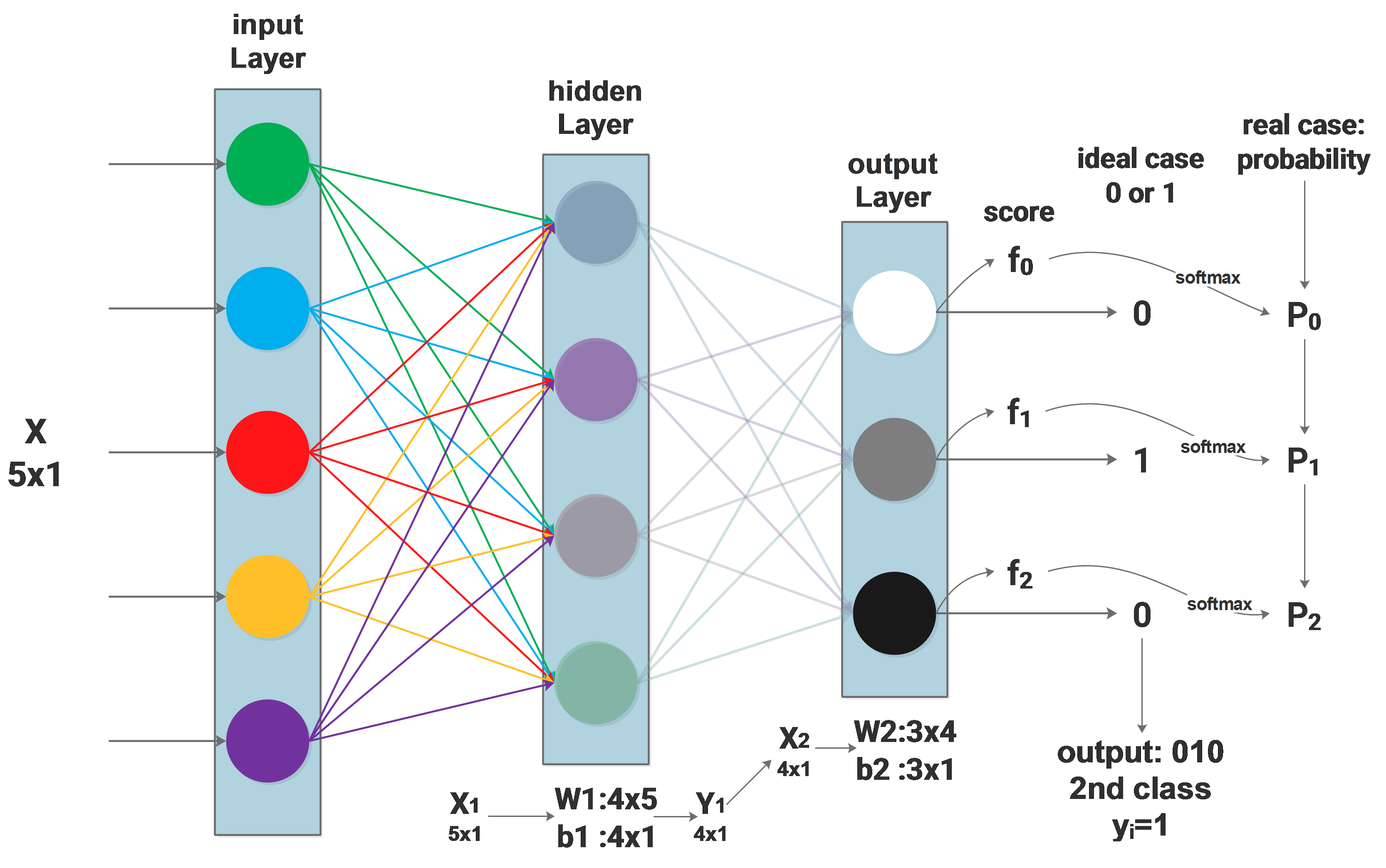
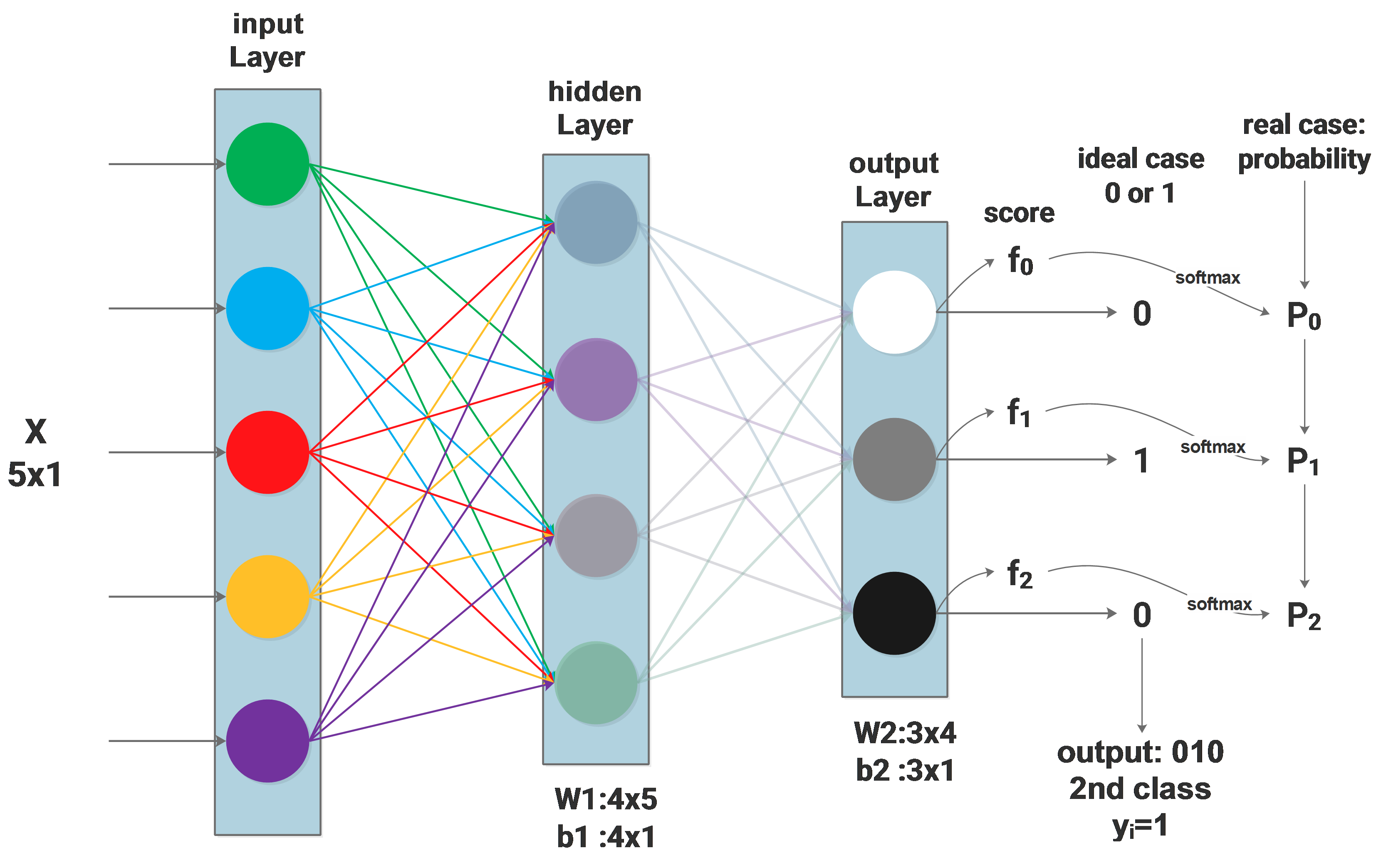
Theoretically, two layer neural network as an universal approximator can fit any random functions. We just need to increase the number of features of the hidden layer to make everything fitted. But the efficiency is very low.

Why deep

According to the paper Topology of deep neural networks, evey layer of a ReLU neural network is try to separate the data points by folding the high dimension manifold. The paper uses the Betti number to measure the distance between the current folded manifold and the final target manifold, it discovered that the works each layers have done are different for different networks.

For shallow networks, most of the folding efforts are done by the last layer. For deep networks, the folding efforts done by each layer are similar. Which means, the works done by each layer of a deep neural networks are relatively simple and easy, but the works to be done by the last layer of a shallow network are complicated and hard.

It is not hard to imagine, the deep neural network solves the problem by abstracting it, which makes the training easier and of higher efficiency.

The deeper, the better?

But it doesn’t mean the deeper is better, the paper Increasing Depth Leads to U-Shaped Test Risk in Over-parameterized Convolutional Networks shows that from the beginning depth really helps the neural network to get better, but once the depth passes a threshold, the network get worse:

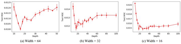
From the left to the right we can see how the test error changes with the change of depth on ResNets of different widths. Obviously, for whatever width, ResNet18 always achieves the best accuracy, and it gets worse after that.

We can understand it in a straight forward way: if the problem is simple, we should not over-abstract it, the networks will be confused by solving a simple problem with too many abstraction. On the other hand, if the problem is very hard, the network needs more layers of abstraction to solve it properly.

Uncertainty estimation of the output from a deep neural network has recently become a hot topic, mainly due to Alex Kendall’s PhD thesis Geometry and Uncertainty in Deep Learning for Computer Vision, where he mentioned the uncertainty problems for semantic and geometrical problems in the computer vision field. What is more, it provides us a weighting strategy for the losses of multi-task learning, which is a very practical problem in both the academical and industrial fields. It is highly recommended to take a close look at Alex Kendall’s presentation of his PhD thesis Geometry and Uncertainty in Deep Learning. As a short introduction of Bayesian deep learning, you can also take a look at his blog article Bayesian deep learning - Alex Kendall.

Come to the topic today, the paper published in ICCV 2019 Gaussian YOLOv3: An Accurate and Fast Object Detector Using Localization Uncertainty for Autonomous Driving tries to apply uncertainty estimation for the detection task, and it succeeded. Uncertainty estimation is much more than uncertainty output, it can also be used to construct a loss function and raise the detection accuracy. The paper focused on estimating the uncertainty of the bounding box localization, which means the coordinate of the bounding box center and its width and height. By using the uncertainty estimation, the paper managed to achieve 3.5 more mAP than the original YoloV3 with 1% more computational cost, what is more, the implementation is also quite straight forward. This blog will provide a in-depth explaination of this paper.

The idea behind PCA

In the field of machine learning, PCA is used to reduce the dimension of features. Usually we collect a lot of feature to feed the machine learning model, we believe that more features provides more information and will lead to better result.

But some of the features doesn’t really bring new information and they are correlated to some other features. PCA is then introduced to remove this correlation by approximating the original data in its subspace, some of the features of the original data may be correlated to each other in its original space, but this correlation doesn’t exit in its subspace approximation.

Visually, let’s assume that our original data points \(x_1...x_m\) have 2 features and they can be visualized in a 2D space:

The case we are handling: a 2 layers network

Background:the network and symbols

Firstly the network architecture will be described as:

Dropout regularization

Dropout is a commonly used regularization method, it can be described by the diagram below: only part of the neurons in the whole network are updated. Mathematically, we apply some possibility \(p\)(we use 0.5) to a neuron to keep it active or keep it asleep:

Weight Initialization

All-Zero Initialization

It is easy to think that we set all the weights to be zero, but it’s terribly wrong, cause using all zero initialization will make the neurons all the same during the backpropagation update. We don’t need so many identical neurons. Actually, this problem always exists if the weights are initialized to be the same.

Small random values

One guess to solve the problem of all-zero initialization is setting the weights to be small random values, such as \(W=0.01*np.random.randn(D,H) ​\) . It is also problematic because very small weights cause very small updates and the update values become smaller and smaller during the backpropagation. In the deep network, this problem is very serious as you may find that the upper layers never update.

The LSVM (SVM with latent variable) is mostly used for human figure detection, it is very efficiency because it puts the human figure’s structure into consideration: a human figure has hands, head and legs. The LSVM models the human figure structure with 6 parts, and the position of these 6 parts are latent value.

The basic logic is sliding a window on the image, for every position we get a small image patch, by scoring this image patch we can predict whether this image patch contains a human figure or not.

Defining the score function

Anyway, the first thing to do: defining a score function:

Structural SVM is a variation of SVM, hereafter to be refered as SSVM

Special prediction function of SSVM

Firstly let’s recall the normal SVM’s prediction function:

\[f(x)=sgn((ω\cdot x)+b)\]

ω is the weight vector，x is the input，b is the bias，\(sgn\) is sign function，\(f(x)\) is the prediction result.

On of SSVM’s specialties is its prediction function：

\[f_ω (x)=argmax_{y∈Υ} [ω\cdot Φ(x,y)]\]

y is the possible prediction result，Υ is y’s searching space，and Φ is some function of x and y.Φ will be a joint feature vector describes the relationship between x and y

Then for some given \(\omega\), different prediction will be made according to different x.

Sepp Hochreiter was graduated from Technische Universität München, LSTM was invented when he was in TU and now he is the head of Institute of Bioinformatics, Johannes Kepler University Linz.

Today he comes by Munich and gives a lecture in Fakultät Informatik.

At first, Hochreiter praised how hot is Deep Learning (to be referred as DL) around the world these days, especially LSTM, which is now used in the new version of google translate published a few days ago. The improvements DL made in the fields of vision and NLP are very impressive.

Then he starts to tell the magic of DL, taking face recognition as an example, the so-called CNN (Convolution Neuro Networks):

Centering and Scaling

Simple Neuron

The above diagram shows a neuron in NN, it simulates a real neuron:

it has inputs: \(x_{0},x_{1}\dots x_{i}\)

it has weights for each inputs: \(\omega_{0},\omega_{1}\dots \omega_{i}\): weight vector

it has bias \(b\)

it has a threshold for the “activation function”

Review

For the ith sample \((x_i,y_i)\) in the training set, we have the following loss function:

\[L_i= \sum_{j≠y_i}max(0,w_j^T\cdot x_i−w_{y_i}^T\cdot x_i+Δ)\]

\(w_j^T\cdot x_i\) is the score classifying \(x_i\) to class j，and \(w_{y_i}^T\cdot x_i\) is the score classifying correctly(classify to class \(y_i\))，\(\omega_i\) is the \(j\)th row of \(W\).

Problem

Problem 1:

Considering the geometrical meaning of the weight vector \(\omega\), it is easy to find out that \(\omega\) is not unique, \(\omega\) can change in a small area and result in the same \(L_i\).

Problem 2:

It the values in \(\omega\) is scaled, the loss computed will also be scaled by the same ratio. Considering a loss of 15, if we scale all the weights in \(\omega\) by 2, the loss will be scaled to 30. But this kind of scaling is meaningless, it doesn’t really represent the loss.

PCA (Principal component analysis), just as its name shows, it computes the data set’s internal structure, its “principal components”.

Considering a set of 2 dimensional data, for one data point, it has 2 dimensions \(x_1\) and \(x_2\) . Now we get n such data points . What is the relationship between the first dimension \(x_1\) and the second dimension \(x_2\) ? We compute the so called covariance:

\[cov(x_1,x_2)=\frac{\displaystyle \sum_{i=1}^n{(x_1^i-\overline{x_1})(x_2^i-\overline{x_2})} }{n-1}\]

the covariance shows how strong is the relationship between \(x_1\) and \(x_2\). Its logic is the same as Chebyshev’s sum inequality:

HoG (Histograms of Oriented Gradients) feature is a kind of feature used for human figure detection. At an age without deep learning, it is the best feature to do this work.

Just as its name described, HoG feature compute the gradients of all pixels of an image patch/block. It computes both the gradient’s magnitude and orientation, that’s why it’s called “oriented”, then it computes the histogram of the oriented gradients by separating them to 9 ranges.

One image block (upper left corner of the image) is combined of 4 cells, one cell owns a 9 bins histogram, so for one image block we get 4 histograms, and all these 4 histograms will be flattened to one feature vector with a length of 4x9. Compute the feature vectors for all blocks in the image, we get a feature vector map.

Taking one pixel (marked red) from the yellow cell as an example: compute the \(\bigtriangledown_x\) and \(\bigtriangledown_y\) of this pixel, then we get its magnitude and orientation(represented by angle). When calculating the histogram, we vote its magnitude to its neighboring 2 bins using bilinear interpolation of angles.

Finally, when we get the 4 histograms of the 4 cells, we normalize them according to the summation of all the 4x9 values.

The details are described in the following chart:

Loss Function

Now we want to solve a image classification problem, for example classifying an image to be cow or cat. The machine learning algorithm will score a unclassified image according to different classes, and decide which class does this image belong to based on the score. One of the keys of the classification algorithm is designing this loss function.

Map/compute image pixels to the confidence score of each class

Assume a training set:

\[(x_i,y_i)\]

\(x_i\) is the image and \(y_i\) is the corresponding class

i∈1…N means the traning set constains N images

\(y_i\)∈1…K means there are K image categories

So a score function maps x to y:

\[f(x_i,W,b)=W\cdot x_i+b\]

In the above function, each image \(x_i\) is flattend to a 1 dimention vector

If one image’s size is 32x32 pixels with 3 channels

\(x_i\) will be a 1 dimention vector with the length of D=32x32x3=3072 Parameter matrix W has the size of [KxD], it is often called weights b of size [Kx1] is often called bias vector In this way, W is evaluating \(x_i\)’s confidence score for K categories at the same time