Gaussian Yolo V3 - get 3.5 more mAP and uncertainty with 1% more computation

Uncertainty estimation of the output from a deep neural network has recently become a hot topic, mainly due to Alex Kendall’s PhD thesis Geometry and Uncertainty in Deep Learning for Computer Vision, where he mentioned the uncertainty problems for semantic and geometrical problems in the computer vision field. What is more, it provides us a weighting strategy for the losses of multi-task learning, which is a very practical problem in both the academical and industrial fields. It is highly recommended to take a close look at Alex Kendall’s presentation of his PhD thesis Geometry and Uncertainty in Deep Learning. As a short introduction of Bayesian deep learning, you can also take a look at his blog article Bayesian deep learning - Alex Kendall.

Come to the topic today, the paper published in ICCV 2019 Gaussian YOLOv3: An Accurate and Fast Object Detector Using Localization Uncertainty for Autonomous Driving tries to apply uncertainty estimation for the detection task, and it succeeded. Uncertainty estimation is much more than uncertainty output, it can also be used to construct a loss function and raise the detection accuracy. The paper focused on estimating the uncertainty of the bounding box localization, which means the coordinate of the bounding box center and its width and height. By using the uncertainty estimation, the paper managed to achieve 3.5 more mAP than the original YoloV3 with 1% more computational cost, what is more, the implementation is also quite straight forward. This blog will provide a in-depth explaination of this paper.

Original Yolo V3

The architecture of the original Yolo V3 looks like this:

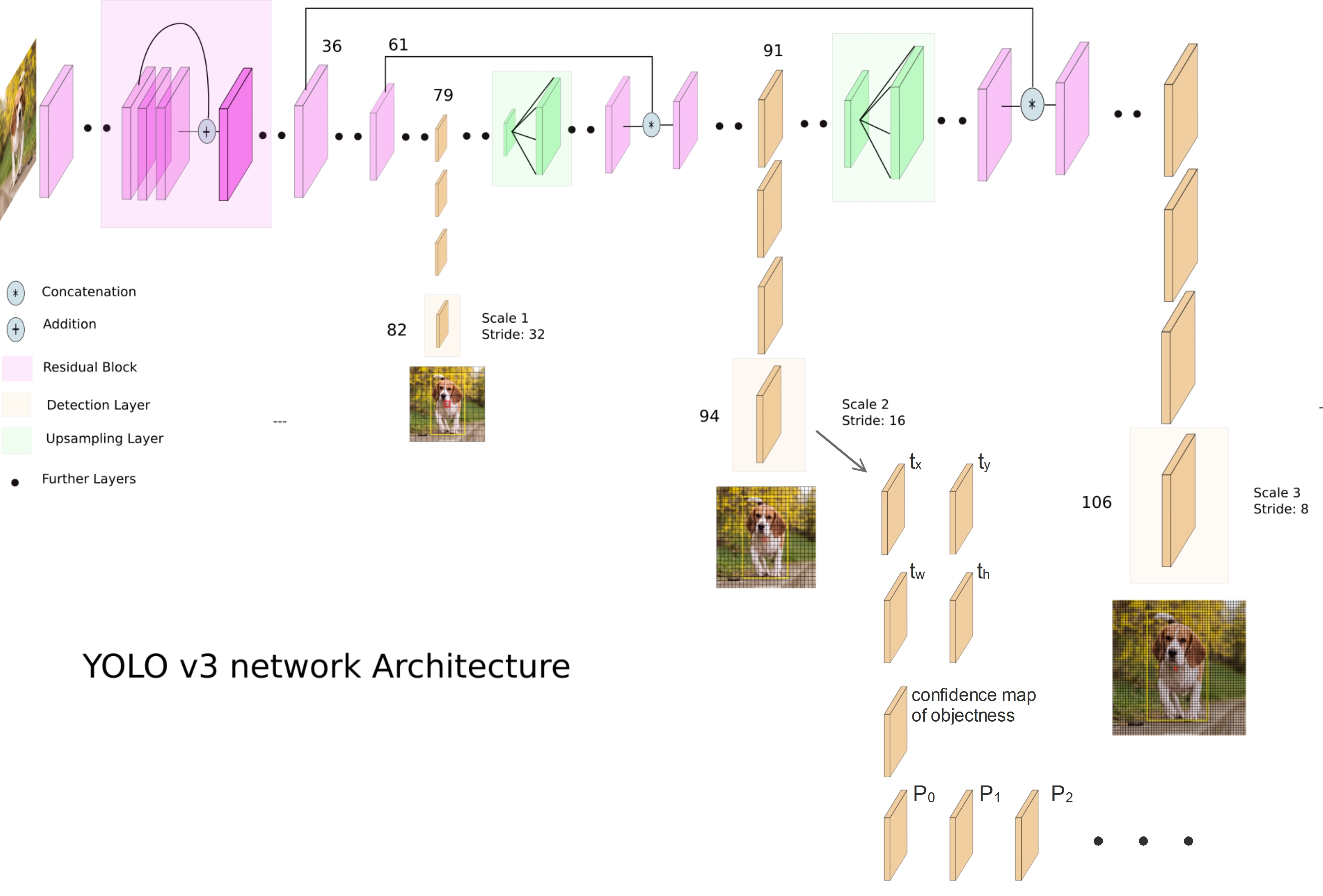
There are detection outputs(Yolo layer) from 3 difference scales, the uncertainty estimation is applied for all 3 Yolo layers, this blog will only explain the Yolo layer of the 2nd scale. The 94th layer consists of the regression channels for bounding box localization(channel \(t_x\) ,\(t_y\), \(t_w\) and \(t_h\)), the confidence map of objectness and the classification channels for different classes(\(P_0\) ,\(P_1\) ….).

Based on the detection encoding of Yolo V3, each pixel of a Yolo layer represent a grid cell, \(t_x\) and \(t_y\) represent the coordinates of the bounding box center within a grid cell, thus their ranges must be between 0 and 1. As an example, if the bounding box center is located at the center of a grid cell, both \(t_x,t_y\) will be 0.5. In order to make sure that the regressed value does not exceed the range, a sigmoid activation layer is used to regress \(t_x, t_y\).

For \(t_w, t_h\), they are used to encode the width and height of the bounding box based on the prior:

\[b_w=p_we^{t_w}\\ b_h=p_he^{t_h}\]

where \(b_w,b_h\) are the predicted bounding box width and height, \(t_w, t_h\) are the direct outputs from the detection layer.

Yolo V3 with uncertainty

With uncertainty output, the meaning of the network output is changed. The network does not only regress the value itself (such as \(t_x, t_y, t_w, t_h\)), it also regresses the uncertainty of these four values. Then the outputs of the network turn to be like this:

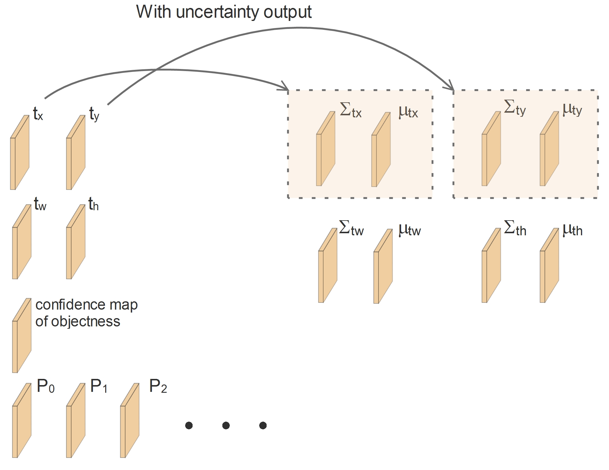
From a probabilistic point of view, we treat the output values as a parameter pair \((\mu, \Sigma)\) which represents a Gaussian distribution. Instead of only predicting a value \(t_x\), the network tries to predict a Gaussian distribution of the value \(t_x\). This Gaussian distribution can be described by its mean \(\mu_{t_x}\) and variance \(\Sigma_{t_x}\):

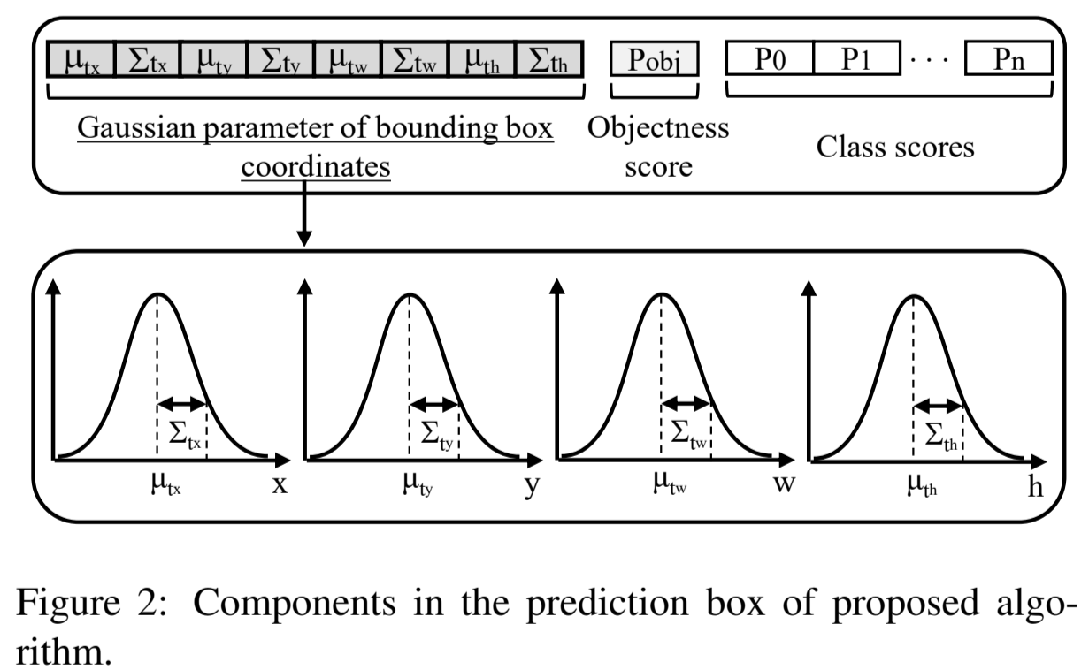
So, the output \((\mu_{tx},\Sigma_{t_x})\) is treated as a complete Gaussian curve. More naturally, we can also treat the mean value \(\mu_{t_x}\) as the prediction \(t_x\) and the variance \(\Sigma_{t_x}\) as its uncertainty.

We should pay attention here that the variance \(\Sigma_{t_x}\) can be interpreted as uncertainty just because the range of the value \(t_x\) is between 0 and 1, therefore its variance will be also in the range of \([0, 1]\). Otherwise, if the variance can be bigger than 1, we will not be able to interpret it as uncertainty.

Usually, the first doubt people have for the prediction with uncertainty is : where can we get the ground truth for the uncertainty \(\Sigma\)?

The answer is simple: we do not need ground truth for the uncertainty, it is learned automatically. Let us assume the uncertainty is part of the property of the network itself, then how can we get the ground truth of the network property even when it is not trained? The network is learning by itself to estimate its own uncertainty.

Practically, the uncertainty can be considered as a learned weighting parameter of the loss and a regularizer. Let us take a look at how the loss function will change by introducing the uncertainty.

Without uncertainty, the loss function can be as simple as:

\[Loss = (t_x^{Gt}-t_x)^2\]

where \(t_x^{Gt}\) is the ground truth and \(t_x\) is the prediction.

With the uncertainty, even the difference between the ground truth and the prediction is the same, our loss can be different, and it makes a lot of sense:

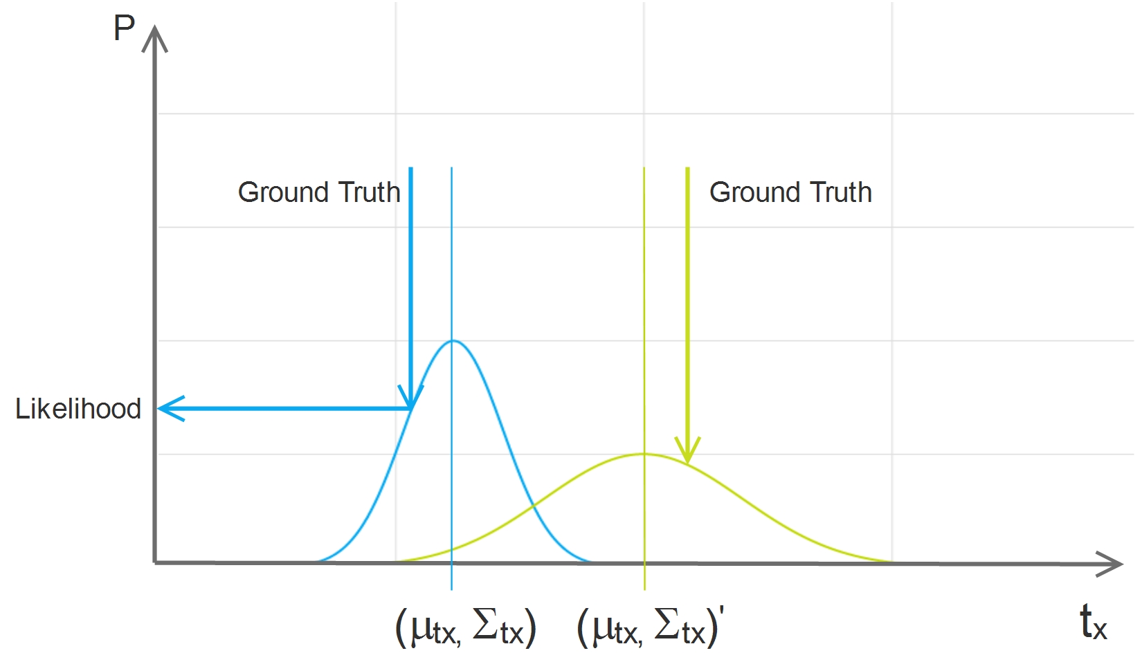
In the above diagram, \(t_x\) has a small uncertainty and \(t_x'\) has a big uncertainty. For both cases, the absolute differences between the ground truth and the prediction are the same, but the likelihood is quite different. It is natural that we can learn more from the loss of very certain output, on the other hand, we would better to keep some doubt on the highly uncertain output.

The concept can be modeled in a simple maximum likelihood framework. Let us say we get a predicted distribution \(\mu_{t_x},\Sigma_{t_x}\), the likelihood of having the ground truth \(t_x^{Gt}\) will be:

\[\displaystyle L(t_x^{Gt}|\mu_{t_x},\Sigma_{t_x})=\frac{1}{\sqrt{2\pi}\Sigma_{t_x}}e^{-\frac{(t_x^{Gt}-\mu_{t_x})^2}{2\Sigma_{t_x}^2}}\]

Just as the classical MLE, we use the negative log-likelihood as our final loss function:

\[Loss=-log(L(t_x^{Gt}|\mu_{t_x},\Sigma_{t_x}))=\frac{(t_x^{Gt}-\mu_{t_x})^2}{2\Sigma_{t_x}^2}+log(\Sigma_{t_x})\]

From the above equation, we can see the uncertainty \(\Sigma_{t_x}\) is used as a weighting factor for the normal squared error.

When the uncertainty is big, the loss will be small, then this output will not contribute much to our learning process.

When the uncertainty is small, the loss will be big, because if the network is quite certain about its output but it is actually wrong, it is a very terrible mistake and the network can learn a lot from this error. We weight this error more to make sure that it contributes a lot to our network.

In other words, during the training, the uncertainty tells us how important is each output from every pixel of the feature map and it controls how much we should learn from the error each pixel made.

That is why, by learning the uncertainty, we can learn from the ground truth in a more sophisticated way and the network can be trained better. This is also reflected in the KPI:

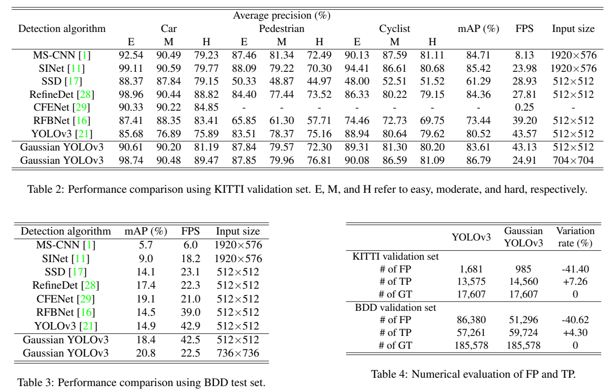
By introducing uncertainty estimation, the mAP rises 3.5 points, it is really a big improvement. And what is more, we get the uncertainty estimation for the localization of each bounding box. The cost is just adding 4 more channels to the Yolo layer, considering we may have more than 100 channels of the Yolo layer and there are many more layers before the Yolo layer, the 1% computation overhead can be ignored.