SVD, PCA and Least Square Problem
The idea behind PCA
In the field of machine learning, PCA is used to reduce the dimension of features. Usually we collect a lot of feature to feed the machine learning model, we believe that more features provides more information and will lead to better result.
But some of the features doesn’t really bring new information and they are correlated to some other features. PCA is then introduced to remove this correlation by approximating the original data in its subspace, some of the features of the original data may be correlated to each other in its original space, but this correlation doesn’t exit in its subspace approximation.
Visually, let’s assume that our original data points \(x_1...x_m\) have 2 features and they can be visualized in a 2D space:
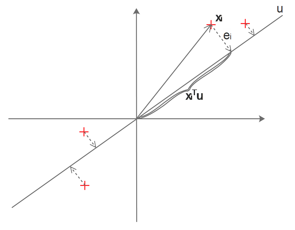
In the above diagram, the red crosses represent our original data points, we want to find a line \(u\), which approximates the original points by projecting then on \(u\).
Which kind of \(u\) can best approximates the points? Naturally, we want the information of the original data points to be kept in the approximated data points, which means to make sure that they are far away from each other.
Mathematically, we want to find the \(u\) which can maximize the variance of the projected data points.
Symbols:
\(x_1 ... x_m\) : \(m\) data points
\(x_i\) : the \(i\)th data point, a 2x1 feature vector containing 2 features
\(u\) : the subspace of \(x\), \(x\) are located in a 2D space, then \(u\) will be a 1D line, parameterized to be a 2x1 vector: \(u\) is a unit directional vector, representing one direction of the \(x\) space.
Before everything, we firstly preprocess the data points by z-score normalization:
Compute the mean of \(x\):
\[\mu =\frac{1}{m} \sum_{i=1}^m{x_i}\]Compute the standard deviation of \(x\):
\[\sigma = \sqrt{\frac{1}{m}\sum_{i=1}^m{(x_i-\mu)^2}}\]z-score normalize every \(x_i\):
\[x_i = \frac{x_i-\mu}{\sigma}\]in order to simplify the symbols, we just update all original \(x\) to be normalized.
Obviously, for a certain \(x_i\), the distance of its projection on \(u\) to the origin will be its dot product with \(u\):
\[||Proj_u(x_i)-0||=x_i^Tu\]As \(x_i\) is already centered, its variance is:
\[Var(x_i) =(x_i^Tu)^2\]Then our goal will be:
\[arg\max_u(\frac{1}{m}\sum_{i=1}^{m}Var(x_i))\\ arg\max_u(\frac{1}{m}\sum_{i=1}^{m}(x_i^Tu)^2)\\ arg\max_u(\frac{1}{m}\sum_{i=1}^{m}(x_i^Tu)^T(x_i^Tu))\\ arg\max_u(\frac{1}{m}\sum_{i=1}^{m}(u^Tx_ix_i^Tu))\\ arg\max_uu^T(\frac{1}{m}\sum_{i=1}^{m}(x_ix_i^T))u\]We want to get rid of the \(m\) in \(\frac{1}{m}\sum_{i=1}^{m}(x_ix_i^T)\) and tread every thing as matrix, in order to do this, we put all \(x_i\) together to form a big feature matrix as the following diagram describes:
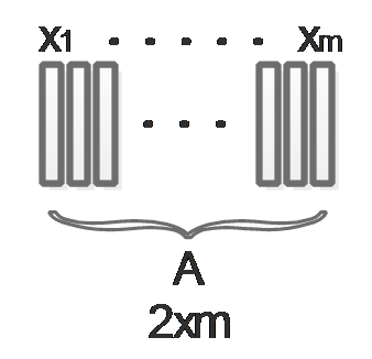
Then \(\frac{1}{m}\sum_{i=1}^{m}(x_ix_i^T)\) turns to be \(AA^T\). Our maximization problem turns to be:
\[arg\max_uu^TAA^Tu\\ arg\min_u-u^TAA^Tu\]Solve it by using Lagrange multiplier and SVD
And we know that \(\|u\|=1\) , this problem can be solved using Lagrange multiplier:
\[\mathcal{L} (u,\lambda)=-u^TAA^Tu+\lambda(u^Tu-1)\]According to the Kuhn-Tucker Conditions, we get:
\[\frac{\partial\mathcal{L} (u,\lambda)}{\partial u}=-\frac{\partial(u^TAA^Tu)}{\partial u}+\frac{\partial(\lambda u^Tu)}{\partial u}=0\\ -2AA^Tu+2\lambda u=0\\ AA^Tu=\lambda u\\\]Obviously, \(u\) and \(\lambda\) are \(AA^T\)’s Eigen vector and Eigen value.
But \(AA^T\) has more than one Eigen vectors, which one should be the \(u\) we are looking for? In order to find it, we replace \(AA^Tu\) in the original equation by \(\lambda u\):
\[u^TAA^Tu=u^T\lambda u=\lambda u^Tu=\lambda\\ arg\max_uu^TAA^Tu=arg\max_u\lambda\]Which means, we can maximize \(u^TAA^Tu\) by simply choosing the biggest Eigen value and its corresponding Eigen vector.
Then we can use SVD to decompose A:
\[A=U\Sigma V^T\]For \(AA^T\), we get:
\[AA^T = U\Sigma V^T( U\Sigma V^T)^T= U\Sigma V^TV\Sigma^TU^T= U\Sigma \Sigma^TU^T\\ AA^TU=U\Sigma \Sigma^TU^TU\\ AA^TU=U\Sigma \Sigma^T\\ AA^TU=\Sigma \Sigma^TU\]Now, as \(\Sigma \Sigma^T\) is a diagonal matrix, we can obviously see that the columns of \(U\) are the Eigen vectors of \(AA^T\) and the diagonal values of \(\Sigma \Sigma^T\) are \(AA^T\)’s Eigen values.
Its relationship to least mean square
As described above, we want to maximize the variance of the projected data points:
\[arg\max_u(\frac{1}{m}\sum_{i=1}^{m}(x_i^Tu)^2)\]Actually, as the \(x_i\) in the above equation are data points which will never change, so it will do no harm to add the following term into the equation:
\[\frac{1}{m}\sum_{i=1}^{m}x_i^2\]Solving the maximization problem is equally solving the following minimization problem:
\[arg\min_u(\frac{1}{m}\sum_{i=1}^{m}x_i^2-\frac{1}{m}\sum_{i=1}^{m}(x_i^Tu)^2)\\ arg\min_u\{\frac{1}{m}\sum_{i=1}^{m}(x_i^2-(x_i^Tu)^2)\}\]Let’s take a look at the diagram again:
Obviously, \(x_i^2-(x_i^Tu)^2\) is actually equal to \(e_i^2\), so our minimization problem turns to:
\[arg\min_u{\frac{1}{m}\sum_{i=1}^{m}e_i^2}\]Which means, we are looking for a line \(u\), which can minimize the summation of the projective distances of the data points onto this line, this is a least mean square error problem. Now we may notice that maximizing the variance is equal to minimizing the mean square.